Parallel and Larger-than-Memory Processing#
Authors: Ian Carroll (NASA, UMBC)
The following notebooks are prerequisites for this tutorial.
Learn with OCI: Data Access
Learn with OCI: Processing with Command-line Tools
Summary#
Processing a whole collection of Ocean Color Instrument (OCI) granules, or even big subsets of that collection, requires breaking up one big job into many small jobs. That and putting the pieces back together again. The reason we break up big jobs has to do with computational resources, specifically memory (i.e. RAM) and processors (i.e. CPUs or GPUs). That big collection of OCI granules can’t all fit in memory; and even if it could, your computation might only use one of several available processors.
This notebook works towards a better understanding of a tool tightly integrated with XArray that is designed to handle the challenges of effectively creating and managing these jobs. The tool is Dask: a Python library for parallel and distributed computing. Before diving into Dask, the notebook gets started with an even more foundational concept for performant computing: using compiled functions that are typically not even written in Python.
Learning Objectives#
At the end of this notebook you will know:
The importance of using high-performance functions to do array operations
How to start a
daskclient for parallel and larger-than-memory pipelinesOne method for interpolating Level-2 “swath” data to a map projection
Contents#
1. Setup#
Begin by importing all of the packages used in this notebook. If your kernel uses an environment defined following the guidance on the tutorials page, then the imports will be successful.
import dask.array as da
from   dask.distributed import Client
import cartopy.crs as ccrs
import earthaccess
from   matplotlib.patches import Rectangle
import matplotlib.pyplot as plt
import numba
import numpy as np
import pyproj
from   scipy.interpolate import griddata
import xarray as xr
from   xarray.backends.api import open_datatree
We will discuss dask in more detail below, but we use several additional packages that are worth their own tutorials:
scipyis a massive collection of useful numerical methods, including a function that resamples irregularly spaced values onto regular (i.e. gridded) coordinatesnumbacan convert many Python functions to make them run fasterpyprojis a database and suite of algorithms for converting between geospatial coordinate reference systems
SatPy is another Python package that could be useful for the processing demonstrated in this notebok, especially through its Pyresample toolking. SatPy requires dedicated readers for any given instrument, however, and no readers have been created for PACE.
Yet another package we are skipping over is rasterio, which is a high-level wrapper for GDAL. Unfortuneately, the GDAL tooling for using “warp” with geolocation arrays has not been released in rasterio.warp.
The data used in the demonstration is the chlor_a product found in the BGC suite of Level-2 ocean color products from OCI.
bbox = (-77, 36, -73, 41)
results = earthaccess.search_data(
    short_name="PACE_OCI_L2_BGC_NRT",
    temporal=(None, "2024-07"),
    bounding_box=bbox,
)
len(results)
238
The search results include all granules from launch through July of 2024 that intersect a bounding box around the Chesapeake and Delaware Bays. The region is much smaller than an OCI swath, so we do not use the cloud cover search filter which considers the whole swath.
results[0]

paths = earthaccess.open(results[:1])
datatree = open_datatree(paths[0])
dataset = xr.merge(datatree.to_dict().values())
dataset = dataset.set_coords(("latitude", "longitude"))
dataset
<xarray.Dataset> Size: 70MB
Dimensions:           (number_of_bands: 286, number_of_reflective_bands: 286,
                       number_of_lines: 1710, pixels_per_line: 1272)
Coordinates:
    longitude         (number_of_lines, pixels_per_line) float32 9MB ...
    latitude          (number_of_lines, pixels_per_line) float32 9MB ...
Dimensions without coordinates: number_of_bands, number_of_reflective_bands,
                                number_of_lines, pixels_per_line
Data variables: (12/28)
    wavelength        (number_of_bands) float64 2kB ...
    vcal_gain         (number_of_reflective_bands) float32 1kB ...
    vcal_offset       (number_of_reflective_bands) float32 1kB ...
    F0                (number_of_reflective_bands) float32 1kB ...
    aw                (number_of_reflective_bands) float32 1kB ...
    bbw               (number_of_reflective_bands) float32 1kB ...
    ...                ...
    carbon_phyto      (number_of_lines, pixels_per_line) float32 9MB ...
    poc               (number_of_lines, pixels_per_line) float32 9MB ...
    chlor_a_unc       (number_of_lines, pixels_per_line) float32 9MB ...
    carbon_phyto_unc  (number_of_lines, pixels_per_line) float32 9MB ...
    l2_flags          (number_of_lines, pixels_per_line) int32 9MB ...
    tilt              (number_of_lines) float32 7kB ...
Attributes: (12/45)
    title:                             OCI Level-2 Data BGC
    product_name:                      PACE_OCI.20240305T163222.L2.OC_BGC.V2_...
    processing_version:                2.0
    history:                           l2gen par=/data10/sdpsoper/vdc/vpu9/wo...
    instrument:                        OCI
    platform:                          PACE
    ...                                ...
    geospatial_lon_max:                -44.237003
    geospatial_lon_min:                -83.810196
    startDirection:                    Ascending
    endDirection:                      Ascending
    day_night_flag:                    Day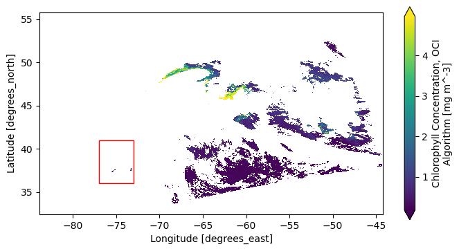
earth_sun_distance_correction: 1.0161924362182617As a reminder, the Level-2 data has latitude and longitude arrays that give the geolocation of every pixel. The number_of_line and pixels_per_line dimensions don’t have any meaningful coordinates that would be useful for stacking Level-2 files over time. In a lot of the granules, like the one visualized here, there will be a tiny amount of data within the box. But we don’t want to lose a single pixel (if we can help it)!
fig = plt.figure(figsize=(8, 4))
axes = fig.add_subplot()
artist = dataset["chlor_a"].plot.pcolormesh(x="longitude", y="latitude", robust=True, ax=axes)
axes.add_patch(Rectangle(bbox[:2], bbox[2]-bbox[0], bbox[3]-bbox[1], edgecolor="red", facecolor="none"))
axes.set_aspect("equal")
plt.show()
When we get to opening mulitple datasets, we will use a helper function to prepare the datasets for concatenation.
def time_from_attr(ds):
    """Set the time attribute as a dataset variable

    Args:
        ds: a dataset corresponding to a Level-2 granule

    Returns:
        the dataset with a scalar "time" coordinate
    """
    datetime = ds.attrs["time_coverage_start"].replace("Z", "")
    ds["time"] = ((), np.datetime64(datetime, "ns"))
    ds = ds.set_coords("time")
    return ds

def trim_number_of_lines(ds):
    ds = ds.isel({"number_of_lines": slice(0, 1709)})
    return ds
Before we get to data, we will play with some random numbers. Whenever you use random numbers, a good practice is to set a fixed but unique seed, such as the result of secrets.randbits(64).
random = np.random.default_rng(seed=5179916885778238210)
2. Compiled Functions#
Before diving in to OCI data, we should discuss two important considerations for when you are trying to improve performance (a.k.a. your processing is taking longer than you would like).
Am I using compiled functions?
Can I use compiled functions in a split-apply-combine pipeline?
When you wrie a function in Python, there is not usually any compilation step like you encounter when writing functions in C/C++ or Fortran. Compilation converts code written in a human-readable language to a machine-readable language. It does this once, and then you use the resulting compiled function repeatedly. That does not happen in Python for added flexibility and ease of programming, but it has a performance cost.
A simple way to measure performance (i.e. speed) in notebooks is to use the IPython %%timeit magic. Begin any cell
with %%timeit on a line by itself to trigger that cell to run many times under a timer and print a summary
of how long it takes the cell to run on average.
%%timeit
n = 10_000
x = 0
for i in range(n):
    x = x + i
x / n
817 μs ± 289 μs per loop (mean ± std. dev. of 7 runs, 1,000 loops each)
The for-loop in that example could be replaced with a compiled function that calculates the mean of a range.
Python is an interpretted language; there is no step during evaluation that compiles code written in Python
to a lower-level language for your operating system. However, we can call functions from packages that
are already compiled, such as the numpy.mean function. In fact, we can even use the numba “just-in-time”
compiler to make our own compiled functions.
When you are interested in performance improvements for data processing, the first tool
in your kit is compiled functions. If you use NumPy, you have already checked this box.
However, since you may sometimes need numba, we’re going to start with a comparison
of functions written in and interpreted by Python with the use of compiled functions.
def mean_and_std(x):
    """Compute sample statistics with a for-loop.

    Args:
      x: One-dimensional array of numbers.

    Returns:
      A 2-tuple with the mean and standard deviation.
    """
    # initialize sum (s) and sum-of-squares (ss)
    s = 0
    ss = 0
    # calculate s and ss by iterating over x
    for i in x:
        s += i
        ss += i**2
    # mean and std. dev. calculations
    n = x.size
    mean = s / n
    variance = (ss / n - mean ** 2) * n / (n - 1)
    return mean, variance ** (1/2)
Confirm the function is working; it should return approximations to the mean and standard deviation parameters of the normal distribution we use to generate the sample.
array = random.normal(1, 2, size=100)
mean_and_std(array)
(0.7304780296630995, 2.0301283010773026)
The approximation isn’t very good for a small sample! We are motivated to use a very big array, say \(10^{4}\) numbers, and will compare performance using different tools.
array = random.normal(1, 2, size=10_000)
%%timeit
mean_and_std(array)
2.84 ms ± 197 μs per loop (mean ± std. dev. of 7 runs, 100 loops each)
On this system, the baseline implementation takes between 2 and 3 milliseconds. The numba.njit method
will attempt to compile a Python function and raise an error if it can’t. The argument to numba.njit
is the Python function, and the return value is the compiled function.
compiled_mean_and_std = numba.njit(mean_and_std)
The actual compilation does not occur until the function is called with an argument. This is how mahine-language works, it needs to
know the type of data coming in before any performance improvements can be realized. As a result, the first call to compiled_mean_and_std
will not seem very fast.
compiled_mean_and_std(array)
(1.0084849501238558, 1.9962951466599286)
But now look at that function go!
%%timeit
compiled_mean_and_std(array)
15.9 μs ± 1.08 μs per loop (mean ± std. dev. of 7 runs, 100,000 loops each)
But why write your own functions when an existing compiled function can do what you need well enough?
%%timeit
array.mean(), array.std(ddof=1)
59.6 μs ± 15.4 μs per loop (mean ± std. dev. of 7 runs, 10,000 loops each)
The takeaway message from this brief introduction is:
numpyis fast because it uses efficient, compiled code to do array operationsnumpymay not have a function that does exactly what you want, so you do havenumba.njitas a fallback
Living with what numpy can already do is usually good enough, even if a custom function could have a small edge in performance. Moreover, what you
can do with numpy you can do with dask.array, and that opens up a lot of opportunity for processing large amounts of data without
writing your own numerical methods.
3. Split-Apply-Combine#
The split-apply-combine framework is everywhere in data processing. A simple case is computing group-wise means on a dataset where one variable defines the group and another variable is what you need to average for each group.
split: divide the array into smaller arrays, one for each group
apply: calculte the mean
combine: reassemble the results into a single (smaller due to aggregation) dataset
The same framework is also used without a natural group by which a dataset should be divided. The split is on equal-sized slices of the original dataset, which we call “chunks”. Rather than a group-wise mean, you could use “chunk-apply-combine” to calculate the grand mean in chunks
chunk: divide the array into smaller arrays, or “chunks”
apply: calculate the mean and sample size of each chunk (i.e. skipping missing values)
combine: combine the size-weighted means to compute the mean of the whole array
The apply and combine steps have to be capable of calculating results on a slice that can be combined to equal the result you would have gotten on the full array. If a computation can be shoved through “chunk-apply-combine” (see also “map-reduce”), then we can process an array that is too big to read into memory at once. We can also distribute the computation across processors or across a cluster of computers.
We can represent the framework visually using a task graph, a collection of functions (nodes) linked through input and output data (edges).
flowchart LR

A(random.normal) -->|array| B(mean_and_std)
The output of the random.normal function becomes the input to the mean_and_std function. We can decide to use chunk-apply-combine
if either:
arrayis going to be larger than available memorymean_and_stdcan be accurately calculated from intermediate results on slices ofarray
By the way, numpy arrays have an nbytes attribute that helps you understand how much memory you may need. Note tha most computations require several times the size of an input array to do the math.
f"{array.nbytes / 2**20} MiB"
'0.0762939453125 MiB'
That’s not a big array. Here’s a “big” 1.0 GiB array.
array = random.normal(1, 2, size=2**27)
print(f"{array.nbytes / 2**30} GiB")
1.0 GiB
It’s still not too big to fit in memory on most laptops. For demonstration, let’s assume we could fit a 1.0 GiB array into memory, but not a 3 GiB array. We will calculate the mean of a 3 GiB array, using 3 splits each of size 1 GiB in a serial pipeline. (Simultaneously calculating the standard deviation is left as an exercise for the reader.)
On this system, the serial approach takes between 8 and 9 seconds.
%%timeit

n = 3
s = 0
for _ in range(n):
    array = random.normal(1, 2, size=2**27)
    s += array.mean()
mean = s / n
8.96 s ± 525 ms per loop (mean ± std. dev. of 7 runs, 1 loop each)
All we were able to implement was serial computation, but we have multiple processors availble. When we visualize the task graph for the computation, it’s apparent that running the calculation serially might not have been the most performant strategy.
%%{ init: { 'flowchart': { 'curve': 'monotoneY' } } }%%

flowchart LR

A(random.normal) -->|array| B(split)
B -->|array_0| C0(apply-mean_and_std)
B -->|array_1| C1(apply-mean_and_std)
B -->|array_2| C2(apply-mean_and_std)
subgraph SCHEDULER
C0
C1
C2
end
C0 -->|result_0| D(combine-mean_and_std)
C1 -->|result_1| D
C2 -->|result_2| D
In this task graph, the mean_and_std deviation function is never used! Somehow, the apply-mean_and_std function and combine-mean_and_std deviation functions have to be defined. This is another part of what Dask provides.
client = Client(processes=False, memory_limit="3 GiB")
client
/srv/conda/envs/notebook/lib/python3.10/site-packages/distributed/node.py:182: UserWarning: Port 8787 is already in use.
Perhaps you already have a cluster running?
Hosting the HTTP server on port 46117 instead
  warnings.warn(
Client
Client-b406a850-54c7-11ef-84a6-ca1b012d51b8
| Connection method: Cluster object | Cluster type: distributed.LocalCluster |
| Dashboard: /user/itcarroll/proxy/46117/status |
Cluster Info
LocalCluster
43c77b3f
| Dashboard: /user/itcarroll/proxy/46117/status | Workers: 1 |
| Total threads: 4 | Total memory: 3.00 GiB |
| Status: running | Using processes: False |
Scheduler Info
Scheduler
Scheduler-0affd443-3397-4daa-9f72-d1127c845a7c
| Comm: inproc://192.168.4.183/1190/1 | Workers: 1 |
| Dashboard: /user/itcarroll/proxy/46117/status | Total threads: 4 |
| Started: Just now | Total memory: 3.00 GiB |
Workers
Worker: 0
| Comm: inproc://192.168.4.183/1190/4 | Total threads: 4 |
| Dashboard: /user/itcarroll/proxy/41675/status | Memory: 3.00 GiB |
| Nanny: None | |
| Local directory: /tmp/dask-scratch-space/worker-7wv6eel4 | |
dask_random = da.random.default_rng(random)
dask_array = dask_random.normal(1, 2, size=3*2**27, chunks="32 MiB")
dask_array
|
||||||||||||||||
dask_array.mean()
|
||||||||||||||||
%%timeit
mean = dask_array.mean().compute()
4.13 s ± 45.8 ms per loop (mean ± std. dev. of 7 runs, 1 loop each)
We just demonstrated two ways of doing larger-than-memory calculations.
Our synchronous implemenation (using a for loop) took the strategy of maximizing the use of available memory while processing one chunk: so we used 1 GiB chunks, requiring 3 chunks to get to a 3 GiB array.
Our concurrent implementation (using dask.array), took the strategy of maximizing the use of available processors: so we used small chunks of 32 MiB, requiring many chunks to get to a 3 GiB array.
The concurrent implementation was a little more than twice as fast.
client.close()
4. Stacking Level-2 Granules#
The integration of XArray and Dask is designed to let you work without doing very much different. Of course, there is still a lot of work to do when writing any processing pipeline on a collection of Level-2 granules. Stacking them over time, for instance, may sound easy but requires resampling the data to a common grid. This section demonstrates one method for stacking Level-2 granules.
Choose a projection for a common grid
Get geographic coordinates that correspond to the projected coordinates
Resample each granule to the new coordinate
Stack results along the time dimension
Use pyproj for the first two steps, noting that the EPSG code of the coordinate reference system (CRS) of the Level-2 files is not recorded in the files. Know that it is the universal default for a CRS with latitudes and longitudes: “EPSG:4326”.
aoi = pyproj.aoi.AreaOfInterest(*bbox)
pyproj.CRS.from_epsg(4326)
<Geographic 2D CRS: EPSG:4326>
Name: WGS 84
Axis Info [ellipsoidal]:
- Lat[north]: Geodetic latitude (degree)
- Lon[east]: Geodetic longitude (degree)
Area of Use:
- name: World.
- bounds: (-180.0, -90.0, 180.0, 90.0)
Datum: World Geodetic System 1984 ensemble
- Ellipsoid: WGS 84
- Prime Meridian: Greenwich
The pyproj database contains all the UTM grids and helps us choose the best one for our AOI.
crs_list = pyproj.database.query_utm_crs_info(datum_name="WGS 84", area_of_interest=aoi, contains=True)
for i in crs_list:
    print(i.auth_name, i.code, ": ", i.name)
EPSG 32618 : WGS 84 / UTM zone 18N
pyproj.CRS.from_epsg(32618)
<Projected CRS: EPSG:32618>
Name: WGS 84 / UTM zone 18N
Axis Info [cartesian]:
- E[east]: Easting (metre)
- N[north]: Northing (metre)
Area of Use:
- name: Between 78°W and 72°W, northern hemisphere between equator and 84°N, onshore and offshore. Bahamas. Canada - Nunavut; Ontario; Quebec. Colombia. Cuba. Ecuador. Greenland. Haiti. Jamaica. Panama. Turks and Caicos Islands. United States (USA). Venezuela.
- bounds: (-78.0, 0.0, -72.0, 84.0)
Coordinate Operation:
- name: UTM zone 18N
- method: Transverse Mercator
Datum: World Geodetic System 1984 ensemble
- Ellipsoid: WGS 84
- Prime Meridian: Greenwich
Note that the axis order for EPSG:4326 is (“Lat”, “Lon”), which is “backwards” from the “X”, “Y” used by EPSG:32618. When we use a CRS transformer, this defines the order of arguments.
t = pyproj.Transformer.from_crs("EPSG:4326", "EPSG:32618", area_of_interest=aoi)
x_min, y_min = t.transform(aoi.south_lat_degree, aoi.west_lon_degree)
x_min, y_min
(319733.3418776203, 3985798.2082585823)
x_max, y_max = t.transform(aoi.north_lat_degree, aoi.east_lon_degree)
x_max, y_max
(668207.8851938072, 4540683.529276577)
Create x, y grid as a new xarray.Dataset but then stack it into a 1D array of points.
x_size = int((x_max - x_min) // 1000)
y_size = int((y_max - y_min) // 1000)
grid_point = xr.Dataset({
    "x": ("x", np.linspace(x_min, x_max, x_size)),
    "y": ("y", np.linspace(y_min, y_max, y_size))
})
grid_point = grid_point.stack({"point": ["x", "y"]})
grid_point
<xarray.Dataset> Size: 5MB
Dimensions:  (point: 192792)
Coordinates:
  * point    (point) object 2MB MultiIndex
  * x        (point) float64 2MB 3.197e+05 3.197e+05 ... 6.682e+05 6.682e+05
  * y        (point) float64 2MB 3.986e+06 3.987e+06 ... 4.54e+06 4.541e+06
Data variables:
*empty*To find corresponding latitudes and longitudes in “EPSG:4326”, do the inverse transformation paying attention to the order of arguments and outputs.
lat, lon = t.transform(grid_point["x"], grid_point["y"], direction="INVERSE")
grid_point["lat"] = ("point", lat)
grid_point["lon"] = ("point", lon)
grid_point
<xarray.Dataset> Size: 8MB
Dimensions:  (point: 192792)
Coordinates:
  * point    (point) object 2MB MultiIndex
  * x        (point) float64 2MB 3.197e+05 3.197e+05 ... 6.682e+05 6.682e+05
  * y        (point) float64 2MB 3.986e+06 3.987e+06 ... 4.54e+06 4.541e+06
Data variables:
    lat      (point) float64 2MB 36.0 36.01 36.02 36.03 ... 40.98 40.99 41.0
lon (point) float64 2MB -77.0 -77.0 -77.0 -77.0 ... -73.0 -73.0 -73.0grid_latlon = grid_point.to_dataarray("axis").transpose("point", ...)
Instead of opening a single granule with xr.open_dataset, open all of the granules with xr.open_mfdataset. Use the time_from_attr function defined above to populate a time coordinate from the attributes on each granule.
paths = earthaccess.open(results[10:20])
kwargs = {"combine": "nested", "concat_dim": "time"}
prod = xr.open_mfdataset(paths, preprocess=time_from_attr, **kwargs)
nav = xr.open_mfdataset(paths, preprocess=trim_number_of_lines, group="navigation_data", **kwargs)
sci = xr.open_mfdataset(paths, preprocess=trim_number_of_lines, group="geophysical_data", **kwargs)
dataset = xr.merge((prod, nav, sci))
dataset
<xarray.Dataset> Size: 696MB
Dimensions:           (time: 10, number_of_lines: 1709, pixels_per_line: 1272)
Coordinates:
  * time              (time) datetime64[ns] 80B 2024-03-09T17:14:28.146000 .....
Dimensions without coordinates: number_of_lines, pixels_per_line
Data variables:
    longitude         (time, number_of_lines, pixels_per_line) float32 87MB dask.array<chunksize=(1, 256, 1272), meta=np.ndarray>
    latitude          (time, number_of_lines, pixels_per_line) float32 87MB dask.array<chunksize=(1, 256, 1272), meta=np.ndarray>
    tilt              (time, number_of_lines) float32 68kB dask.array<chunksize=(1, 32), meta=np.ndarray>
    chlor_a           (time, number_of_lines, pixels_per_line) float32 87MB dask.array<chunksize=(1, 256, 1272), meta=np.ndarray>
    carbon_phyto      (time, number_of_lines, pixels_per_line) float32 87MB dask.array<chunksize=(1, 256, 1272), meta=np.ndarray>
    poc               (time, number_of_lines, pixels_per_line) float32 87MB dask.array<chunksize=(1, 256, 1272), meta=np.ndarray>
    chlor_a_unc       (time, number_of_lines, pixels_per_line) float32 87MB dask.array<chunksize=(1, 256, 1272), meta=np.ndarray>
    carbon_phyto_unc  (time, number_of_lines, pixels_per_line) float32 87MB dask.array<chunksize=(1, 256, 1272), meta=np.ndarray>
    l2_flags          (time, number_of_lines, pixels_per_line) int32 87MB dask.array<chunksize=(1, 256, 1272), meta=np.ndarray>
Attributes: (12/45)
    title:                             OCI Level-2 Data BGC
    product_name:                      PACE_OCI.20240309T171428.L2.OC_BGC.V2_...
    processing_version:                2.0
    history:                           l2gen par=/data11/sdpsoper/vdc/vpu10/w...
    instrument:                        OCI
    platform:                          PACE
    ...                                ...
    geospatial_lon_max:                -54.788364
    geospatial_lon_min:                -95.488335
    startDirection:                    Ascending
    endDirection:                      Ascending
    day_night_flag:                    Day
earth_sun_distance_correction: 1.014057993888855Notice that using xr.open_mfdataset automatically triggers the use of dask.array instead of numpy for the variables. To get a dashboard, load up the Dask client.
client = Client(processes=False)
client
/srv/conda/envs/notebook/lib/python3.10/site-packages/distributed/node.py:182: UserWarning: Port 8787 is already in use.
Perhaps you already have a cluster running?
Hosting the HTTP server on port 37981 instead
  warnings.warn(
Client
Client-d5b8a840-54c7-11ef-84a6-ca1b012d51b8
| Connection method: Cluster object | Cluster type: distributed.LocalCluster |
| Dashboard: /user/itcarroll/proxy/37981/status |
Cluster Info
LocalCluster
b768132b
| Dashboard: /user/itcarroll/proxy/37981/status | Workers: 1 |
| Total threads: 4 | Total memory: 7.42 GiB |
| Status: running | Using processes: False |
Scheduler Info
Scheduler
Scheduler-107bfa68-2cf7-4ab5-af9c-36f9245f3f49
| Comm: inproc://192.168.4.183/1190/10 | Workers: 1 |
| Dashboard: /user/itcarroll/proxy/37981/status | Total threads: 4 |
| Started: Just now | Total memory: 7.42 GiB |
Workers
Worker: 0
| Comm: inproc://192.168.4.183/1190/13 | Total threads: 4 |
| Dashboard: /user/itcarroll/proxy/41169/status | Memory: 7.42 GiB |
| Nanny: None | |
| Local directory: /tmp/dask-scratch-space/worker-r22ngheb | |
Disclaimer: the most generic function that we have available to resample the dataset is scipy.interpolate.griddata. This is not specialized for geospatial resampling, so there is likely a better way to do this using pyresample or rasterio.warp.
Due to limitations of griddata however, we have to work in a loop. For each slice over the time dimension (i.e. each file), the loop is going to collect that latitudesa and longitudes as swath_latlon, resample to grid_latlon (which has regular spacing in the projected CRS), and store the result in a list of xr.DataArray.
groups = []
for key, value in dataset.groupby("time"):
    value = value.squeeze("time")
    swath_pixel = value.stack({"point": ["number_of_lines", "pixels_per_line"]}, create_index=False)
    swath_latlon = swath_pixel[["latitude", "longitude"]].to_dataarray("axis").transpose("point", ...)
    gridded = griddata(swath_latlon, swath_pixel["chlor_a"], grid_latlon)
    gridded = xr.DataArray(gridded, dims="point")
    gridded = gridded.expand_dims({"time": [key]})
    groups.append(gridded)
groups[-1]
<xarray.DataArray (time: 1, point: 192792)> Size: 2MB
array([[       nan,        nan,        nan, ...,        nan, 1.3311725 ,
        1.96276935]])
Coordinates:
  * time     (time) datetime64[ns] 8B 2024-03-16T17:58:34.137000
Dimensions without coordinates: pointThen there is the final step of getting the whole collection concatenated together and associated with the projected CRS (the x and y coordinates).
grid_point["chlor_a"] = xr.concat(groups, dim="time")
dataset = grid_point.unstack()
dataset
<xarray.Dataset> Size: 19MB
Dimensions:  (x: 348, y: 554, time: 10)
Coordinates:
  * x        (x) float64 3kB 3.197e+05 3.207e+05 ... 6.672e+05 6.682e+05
  * y        (y) float64 4kB 3.986e+06 3.987e+06 ... 4.54e+06 4.541e+06
  * time     (time) datetime64[ns] 80B 2024-03-09T17:14:28.146000 ... 2024-03...
Data variables:
    lat      (x, y) float64 2MB 36.0 36.01 36.02 36.03 ... 40.98 40.99 41.0
    lon      (x, y) float64 2MB -77.0 -77.0 -77.0 -77.0 ... -73.0 -73.0 -73.0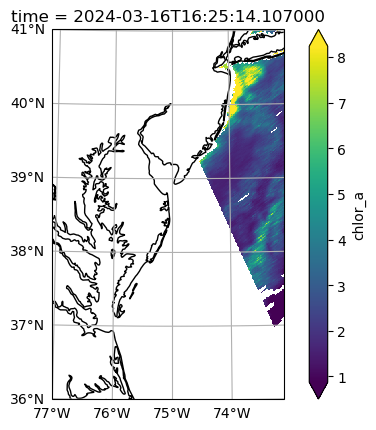
chlor_a (time, x, y) float64 15MB nan nan nan nan ... nan nan 1.331 1.963After viewing a map at individual time slices in projected coordinates, you can decide what to do for your next step of analysis. Some of the granules will have good coverage, free of clouds.
dataset_t = dataset.isel({"time": 4})
fig = plt.figure()
crs = ccrs.UTM(18, southern_hemisphere=False)
axes = plt.axes(projection=crs)
artist = dataset_t["chlor_a"].plot.imshow(x="x", y="y", robust=True, ax=axes)
axes.gridlines(draw_labels={"left": "y", "bottom": "x"})
axes.coastlines()
plt.show()
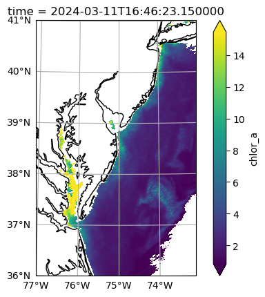
Many will not, either because of clouds or because only some portion of the specified bounding box is within the given swath.
dataset_t = dataset.isel({"time": 8})

fig = plt.figure()
crs = ccrs.UTM(18, southern_hemisphere=False)
axes = plt.axes(projection=crs)
artist = dataset_t["chlor_a"].plot.imshow(x="x", y="y", robust=True, ax=axes)
axes.gridlines(draw_labels={"left": "y", "bottom": "x"})
axes.coastlines()
plt.show()